Grade Adjusted Pace estimates how fast you would have run on a flat route even if your run was on varied grades.
Published
November 17, 2025
Disclaimer
This article is an independent technical-writing sample created solely for portfolio and demonstration purposes.
It is not affiliated with, endorsed by, or produced on behalf of Strava.
All explanations of Grade Adjusted Pace (GAP), its behaviour, and its underlying logic are my own interpretations based on publicly available Strava documentation, Strava Engineering blog posts, and the academic research cited in the bibliography below.
All datasets, adjustment factors, charts, and code shown here are synthetic examples created by me for illustration only. They should not be interpreted as precise reproductions of Strava’s proprietary data or algorithms.
Certain stylistic elements—such as layout choices, callout boxes, metadata fields like “Last modified,” and the overall structure—intentionally emulate the conventions of corporate technical blogs and documentation. These are used purely to demonstrate writing style and document design and should not be taken to imply authorship by Strava or access to internal systems.
Last modified: 17 November 2025
Grade Adjusted Pace (GAP) estimates how fast you would have run on a flat route even if your run was actually on uphill, downhill or mixed grade terrain. By using GAP, runners can better compare paces across routes that have very different terrain profiles.
Note
GAP is a Premium Feature available only to subscribers. You can subscribe here or check out more of our advanced, subscriber-only metrics like Relative Effort here.
You can check your run’s GAP on both the Strava website and the mobile app (Android / iOS). You’ll find it in the following places:
To Do
[Get side-by-side screenshot of the GAP metric on a post-run analysis screen. There would be captions under each image: ‘Mobile View ’on the left, ’Desktop View’ on the right]
Your run’s analysis screen lets you evaluate your GAP across your full activity. You can even zoom in on key points for a closer look at your adjusted pace on any particularly nasty uphills.
Your followers will also be able to view your GAP, so they can see how hard you really worked and give you the compliments you deserve.
How GAP Works
The GAP model uses two inputs: the grade of the terrain and the pace adjustment factor derived from physiological research.
Grade:
Strava estimates the grade (steepness) throughout your run by using elevation data.
See also: Elevation
Pace Adjustment Factor:
Strava’s Grade Adjusted Pace formula is based on research published in the Journal of Applied Physiology by Davies [@Davies1974; @Davies1980] and Minetti [@Minetti2002]. Over time, Strava’s engineering team has continued to build upon these studies. Broadly, the conclusions are:
Effort is affected by the direction of steepness. Positive grades increase effort. Negative grades decrease it.
Effort is affected by the level of steepness. In general, higher levels of steepness have larger effects on effort.
Crucially, however, Strava’s analysis of athlete heart rate data has helped to quantify how much extra effort is expended on uphills or saved on downhills. For example, they found that:
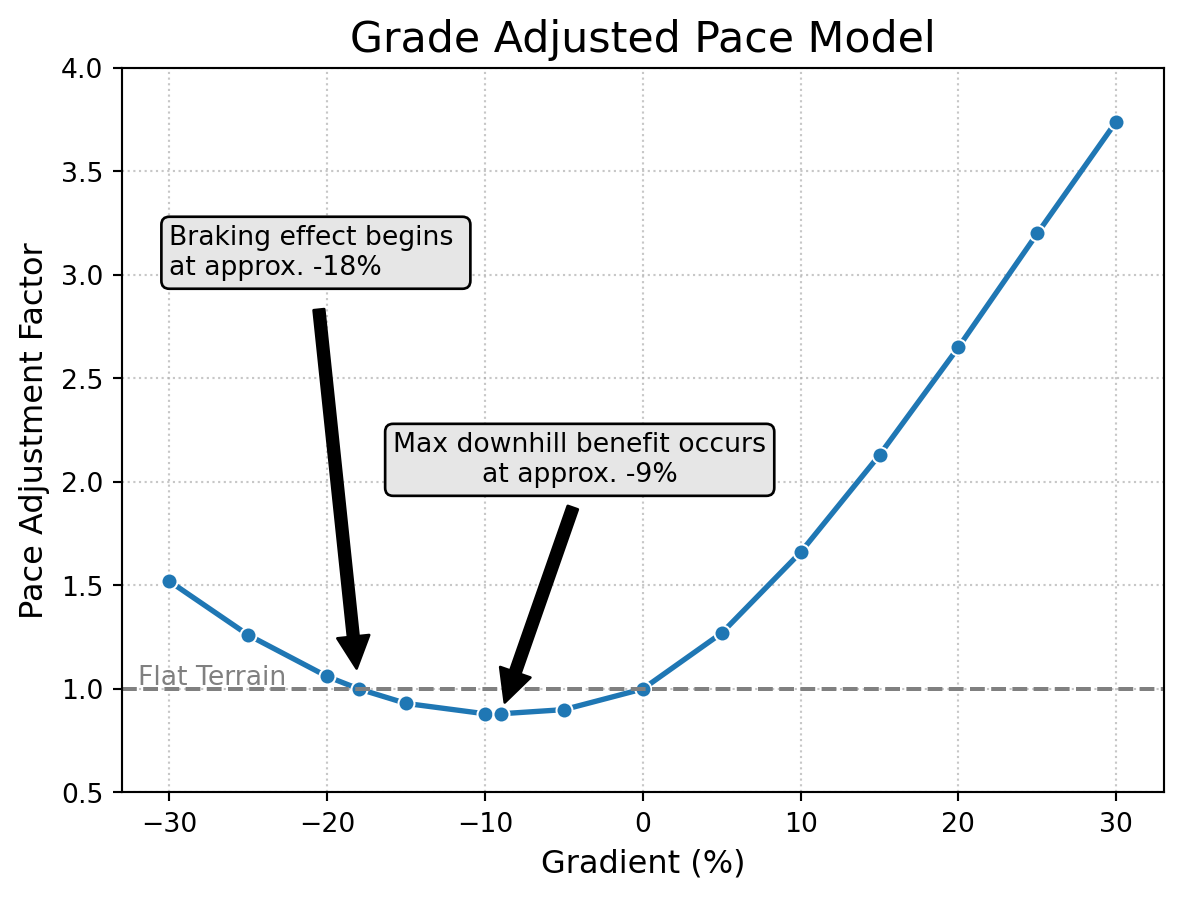
Downhills provide their greatest energy savings and pace increases at grades around -10%. Steeper than this, the positive effects begin to decrease.
At -18% downhills actually have a negative impact on your pace. This is because of a braking effect where runners must actively slow down.
By quantifying the relationship between effort and grade, Strava can apply a Pace Adjustment Factor that is based on grade. On perfectly flat 0% grade terrain, this factor will be 1.0.
The full range of adjustment factors that Strava applies to grades from -30% to +30% can be seen on this graph:
Code
import pandas as pdimport seaborn as snsimport matplotlib.pyplot as plt# 1. Create the example datadata = {'grade_percent': [-30, -25, -20, -18, -15, -10, -9, -5, 0, 5, 10, 15, 20, 25, 30 ],'adjustment_factor': [1.52, 1.26, 1.06, 1.0, 0.93, 0.88, 0.88, 0.9, 1.0, 1.27, 1.66, 2.13, 2.65, 3.2, 3.74 ]}# 2. Create a DataFramedf = pd.DataFrame(data)# 3. Plotfig, ax = plt.subplots()sns.lineplot( data=df, x='grade_percent', y='adjustment_factor', marker='o', # Add markers for the data points lw=2, # Line width ax=ax # Tell seaborn to use our 'ax' object)ax.set_ylim(0.5, 4)ax.set_title('Grade Adjusted Pace Model', fontsize=16)ax.set_xlabel('Gradient (%)', fontsize=12)ax.set_ylabel('Pace Adjustment Factor', fontsize=12)# --- Add a reference line for "flat" ---ax.axhline( y=1.0, color='grey', linestyle='--', lw=1.5)ax.text(-32, 1.02, 'Flat Terrain', color='grey', fontsize=10)# --- Add callouts for key points ---ax.annotate('Max downhill benefit occurs\nat approx. -9%',xy=(-9, 0.88), ha='center', arrowprops=dict(facecolor='black', shrink=0.05), xytext=(-4, 2), fontsize=10, color='black', bbox=dict(boxstyle='round', fc='0.9'))ax.annotate('Braking effect begins \nat approx. -18%',xy=(-18, 1.0), ha='left', arrowprops=dict(facecolor='black', shrink=0.05), xytext=(-30, 3), fontsize=10, color='black', bbox=dict(boxstyle='round', fc='0.9'))# --- Final touches ---ax.grid(True, linestyle=':', alpha=0.7)# --- Use as thumbnail ---fig.savefig("featured.png", facecolor='white')
Figure 1: Strava’s GAP model, showing pace adjustment factor vs. grade.
To understand how the graph works, let’s look at the GAP calculations for a 7 minute mile run on a 5% gradient:
1. Convert minutes/mile to seconds: \(7 × 60 = 420\)
2. Divide by the uphill factor: \(420 ÷ 1.27 ≈ 331\)
3. Convert back to minutes: \(331 ÷ 60 ≈ 5:31\)
The following table shows GAP values for common paces across different gradients.
Grade %
Factor
6:00 mile
7:00 mile
8:00 mile
-7.5
0.89
06:45
07:53
09:01
-5.0
0.90
06:40
07:47
08:53
-2.5
0.95
06:19
07:22
08:25
0.0
1.00
06:00
07:00
08:00
+2.5
1.14
05:16
06:09
07:01
+5.0
1.27
04:44
05:31
06:18
+7.5
1.47
04:05
04:46
05:27
Note
GAP and Pace are identical on flat surfaces
How to Interpret
🔺 SCENARIO 1: You ran a net UPHILL route
Average Grade: +5.0% Factor: 1.27 Pace: 7:00/mile GAP: 5:31/mile
Your pace was divided by a factor greater than 1 when you ran on uphill sections. This meant your GAP was faster than your Pace.
⚡ SCENARIO 2: You ran a net DOWNHILL route
Average Grade: −5.0% Factor: 0.90 Pace: 7:00/mile GAP: 7:47/mile
Your pace was divided by a factor less than 1 when you ran on downhill sections. This meant your GAP was slower than your Pace.
⚖️ SCENARIO 3: You ran a FLAT or BALANCED route
Average Grade: 0% Factor: 1.0 Pace: 7:00/mile GAP: 7:00/mile
Your pace was divided by 1 so it didn’t change.
Tip
Always check the elevation data. A route with constant ups and downs would be very tiring but could still result in a GAP which appears as if it were flat. For example, the Boston Marathon is notoriously challenging due to its uphill sections but is actually a net downhill course.
Limitations
GAP may indicate that a route was flat when it contained significant uphill and downhill sections.
GAP does not adjust for the fatigue caused by effort spikes or uneven pacing on undulating terrain.
GAP does not adjust for any other terrain features or technical difficulties, such as gravel. It only accounts for the gradient.
GAP does not adjust for the additional stress on joints of downhill running.
Golden Rules
GAP is a helpful training tool. You can make more accurate assessments of your fitness level by minimising the confusion caused by hilly terrain. Just follow these golden rules to use it properly.
Use GAP when:
Comparing your best 5 km times on different routes
Assessing fitness trends when you run on varied terrain
Benchmarking tempo run or interval times on new routes by comparing them to your old or existing routes
You have checked the Elevation profile to check if the route is Flat or Balanced
Don’t rely on GAP when:
Running technical trails
Evaluating injury risk from downhills
Measuring pacing discipline
References
To Do
[Fix the quarto bibtex referencing. It’s not working for some reason]