Downloadable attendance churn dataset and walkthrough of its creation - from messy and manual Excel to a tidy and reproducible Python pipeline.
Football
Analytics
Data Engineering
Author
Diggy
Published
January 15, 2026
Introduction
In pandas (and tidy-data workflows), melt() is the standard tool for reshaping a wide table into a long one.
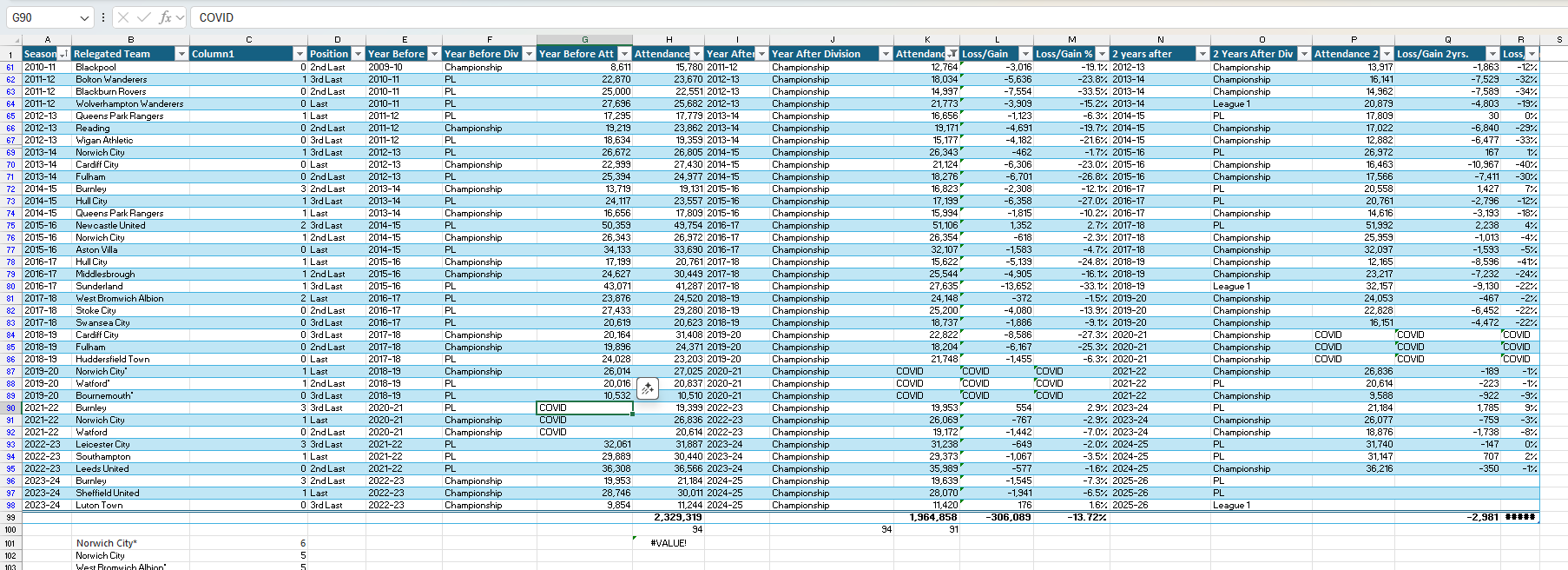
In this project, the original spreadsheet (see below) wasn’t just wide — it was inconsistent across season formats, team naming conventions, and placeholder values (e.g., COVID). A naive pd.melt() would have produced incorrect joins and silent errors.
Unusably messy attendance spreadsheet
This page documents the reproducible reshaping pipeline used to build the final open dataset.
The final output of this process is the perfect_tidy_data.csv file. Read on to learn more about its structure, contents and composition or simply Download perfect_tidy_data.csv. The CSV becomes an analysis-ready Python DataFrame after some further enrichment - see the final code block for details.
Dataset Scope
All Premier League relegations with usable attendance data. This means Covid seasons are excluded. Each Premier League relegation event is represented across a consistent four-season window and includes league performance as well as attendance figures. Data is on a per-season basis, not per-match. - Year -1: Season before relegation
- Year 0: Relegation season (Premier League)
- Year +1: First post-relegation season
- Year +2: Second post-relegation season
A temporary Year +3 is generated programmatically only to determine the Year +2 season outcome (Promoted / Survived / Relegated). After outcome extraction, the Year +3 rows are dropped.
Granularity is one row per team × season × relegation event. So one relegation event (e.g., Burnley 2023-24) is represented by four rows (Year -1 through Year +2).
Data sources
Attendance data
Attendance values were manually compiled into an Excel workbook using:
Because COVID-affected seasons are not comparable to normal seasons, I sometimes entered the string value COVID into attendance cells during manual compilation. The pipeline converts these placeholders to missing values (pd.NA) before numeric conversion.
League tier, final position, and raw season performance totals come from:
The Fjelstul English Football Database (standings dataset)
Fjelstul, Joshua C. “The Fjelstul English Football Database v1.1.0.” May 26, 2024. https://www.github.com/jfjelstul/englishfootball
Licensing note: The Fjelstul database is distributed under CC-BY-SA 4.0. This derived dataset is made available under the same CC BY-SA 4.0 license.
Patch file
The Fjelstul dataset does not include the 2024/25 season, so I have supplemented it with a patch file (standings24_25.csv) to include the most recent completed season.
This identifier is repeated across the four rows representing Year -1 through Year +2.
Reshaping pipeline
Step 0: Prerequisites
import pandas as pdimport numpy as np# You may need to install thefuzzpip install thefuzzfrom thefuzz import process
Step 1 — Load the wide spreadsheet and clean attendance columns
Why: The attendance sheet is wide-format, and attendance values include commas and placeholders (e.g., COVID).
What happens: - Strip commas (e.g., 23,721 → 23721) - Convert COVID and nan placeholders to missing values (pd.NA) - Coerce to numeric
attendance_cols = [c for c in df_wide.columns if"Attendance"in c]for col in attendance_cols: df_wide[col] = df_wide[col].astype(str).str.replace(',', '').replace('COVID', pd.NA).replace('nan', pd.NA) df_wide[col] = pd.to_numeric(df_wide[col], errors='coerce')
Step 2 — Load standings data (for auditing + enrichment)
Why: Team naming mismatches and season key mismatches can silently break merges. The standings dataset provides a stable reference list of teams and seasons.
What happens: - Load standings.csv - Optionally append standings24_25.csv - Rename and select relevant columns - Coerce numeric columns
try:# Load 'season' as string to be safe df_history = pd.read_csv('../../assets/files/datasets/standings.csv', dtype={'season': str})# --- Load patch file and combine ---try: df_patch = pd.read_csv('../../assets/files/datasets/standings24_25.csv', dtype={'season': str})# Append patch data to history data df_history = pd.concat([df_history, df_patch], ignore_index=True)print("Step 2a: Loaded and applied 'standings24_25.csv'.")exceptFileNotFoundError:print("Step 2a: 'standings24_25.csv' not found. Skipping patch.")# --- End new patch logic ---print("Step 2b: Loaded historical data for auditing.")# Create the cleaned df_positions here for later use df_positions = df_history.rename(columns={'team_name': 'Team','season': 'Season','position': 'Position_History','played': 'Games_Played_History','wins': 'Wins_History','goals_for': 'Goals_For_History','goals_against': 'Goals_Against_History','points': 'Points_History','tier': 'Tier_History' })[['Team', 'Season', 'Position_History', 'Games_Played_History', 'Wins_History','Goals_For_History', 'Goals_Against_History', 'Points_History', 'Tier_History']]# Convert new history columns to numeric numeric_cols = ['Position_History', 'Games_Played_History', 'Wins_History','Goals_For_History', 'Goals_Against_History', 'Points_History', 'Tier_History']for col in numeric_cols: df_positions[col] = pd.to_numeric(df_positions[col], errors='coerce')
Step 3 — Audit team names (fuzzy matching)
Why: The manual spreadsheet uses informal names (Man City, Spurs, etc.). The merge requires standardized names.
What happens:
- Identify team names in attendance sheet that don’t match standings - Propose high-confidence fuzzy matches (>85) - Warn on low-confidence values
teams_in_wide_df =set(df_wide['Relegated Team'].astype(str).unique()) teams_in_history_df =set(df_positions['Team'].astype(str).unique()) unmatched_teams = teams_in_wide_df.difference(teams_in_history_df)# Create an empty map to build automatically auto_team_name_map = {}if unmatched_teams:print("--- AUDIT: TEAM NAME MISMATCHES FOUND ---")print("The following teams from your file do not match the history file.")print("Attempting to build an automatic mapping...")# Loop through each unique unmatched team and find the best matchfor team insorted(unmatched_teams):# process.extractOne returns a tuple: (best_match, score) suggestion = process.extractOne(team, teams_in_history_df)# Auto-map spaces, asterisks, and high-confidence matchesif suggestion[1] >85:print(f" - Auto-mapping: \"{team}\" -> \"{suggestion[0]}\" (Score: {suggestion[1]})") auto_team_name_map[team] = suggestion[0]else:# Don't map low-confidence or junk dataif team notin ['nan', 'TEAM', 'Relegated Team']:print(f" - WARNING: \"{team}\" has no confident match. (Best: \"{suggestion[0]}\" at {suggestion[1]}%)")print(f" -> Please add a fix for \"{team}\" to 'manual_overrides_map' in Step 4.")print("---------------------------------------------")else:print("--- AUDIT: TEAM NAMES OK ---")print("All team names in your file match the history file.")exceptFileNotFoundError:print("Error: '../../assets/files/datasets/standings.csv' not found. Skipping audit and enrichment.")# Create empty dataframes if file not found df_positions = pd.DataFrame(columns=['Team', 'Season', 'Position_History', 'Games_Played_History','Wins_History', 'Goals_For_History', 'Goals_Against_History','Points_History', 'Tier_History']) auto_team_name_map = {}
Step 4 — Standardize team names (auto-map + manual overrides)
Why: Fuzzy matching is helpful but not perfect; known edge cases are fixed with manual overrides.
What happens: - Merge the auto-map and manual overrides
- Replace names in the wide spreadsheet
- Filter out remaining junk/unmapped rows
manual_overrides_map = {"Man Utd": "Manchester United","Man City": "Manchester City","Spurs": "Tottenham Hotspur","QPR": "Queens Park Rangers","Wolves": "Wolverhampton Wanderers","Sheff Utd": "Sheffield United","Sheff Wed": "Sheffield Wednesday","Nott'm Forest": "Nottingham Forest","Notts County": "Nottingham Forest"# e.g., if audit warns about "Bradford", add:# "Bradford": "Bradford City",}# Combine the auto-generated map with the manual overrides# This is where we combine the two dictionaries.# The 'manual_overrides_map' will overwrite any conflicting keys from 'auto_team_name_map'.final_team_map = {**auto_team_name_map, **manual_overrides_map}df_wide['Relegated Team'] = df_wide['Relegated Team'].replace(final_team_map)print("Step 4: Standardized 'Relegated Team' names using auto-mapping and manual overrides.")# --- 4.5. FILTERING STEP ---# Now that names are mapped, we can filter out junk rows that didn't get mappedteams_in_history_df =set(df_positions['Team'].astype(str).unique())df_wide = df_wide[df_wide['Relegated Team'].isin(teams_in_history_df)]print("Step 4.5: Filtered out junk rows (e.g., 'nan', 'TEAM').")
Step 5 — Create a stable event key (Relegation_Event_ID)
Why: Each relegation event needs a stable identifier across Year -1..+2.
df_wide['Relegation_Event_ID'] = df_wide['Relegated Team'] +' '+ df_wide['Season']print("Step 5: Created 'Relegation_Event_ID'.")
Why: The attendance sheet is wide and not safely meltable without careful column mapping.
What happens:
- Create four normalized slices (Year -1..+2)
- Concatenate into one long table with a consistent schema
## Helper function to create each slicedef make_slice(df, team_col, season_col, att_col, year_vs):# --- Check if att_col exists, otherwise use pd.NA ---# This makes the function robust for the missing Y3 attendanceif att_col notin df.columns:# Create a temporary column of NAs if the attendance col doesn't exist df = df.assign(Attendance_tmp=pd.NA) else:# If the col *does* exist, rename it df = df.rename(columns={att_col: "Attendance_tmp"}) slice_df = df.rename(columns={ team_col: "Team", season_col: "Season_tmp" }).assign(Year_vs_Relegation=year_vs)# Select and rename final columns slice_df = slice_df[['Relegation_Event_ID', 'Team', 'Season_tmp', 'Attendance_tmp', 'Year_vs_Relegation']].copy() slice_df.columns = ['Relegation_Event_ID', 'Team', 'Season', 'Attendance', 'Year_vs_Relegation']return slice_df# Create slices (Only up to Year 2)slice_minus1 = make_slice(df_wide, "Relegated Team", "Year Before", "Year Before Att", -1)slice_0 = make_slice(df_wide, "Relegated Team", "Season", "Attendance", 0)slice_1 = make_slice(df_wide, "Relegated Team", "Year After", "Attendance year after", 1)slice_2 = make_slice(df_wide, "Relegated Team", "2 years after", "Attendance 2 years after", 2)# Concatenate slices safelydf_tidy = pd.concat([slice_minus1, slice_0, slice_1, slice_2], ignore_index=True)print("Step 6: Data has been 'tidied' successfully!")
Step 7 — Standardize season keys (YYYY-YY)
Why: Season formats vary (e.g., 1991-1992 vs 1992-93) and must align for joins.
# --- HELPER FUNCTION 1 ---def format_season(season_str):"""Converts '1991-1992' to '1991-92' and leaves '1992-93' as is."""if pd.isna(season_str):return pd.NA parts =str(season_str).split('-')iflen(parts) ==2:iflen(parts[1]) ==4: # Format is '1991-1992'returnf"{parts[0]}-{parts[1][-2:]}"else: # Format is '1992-93'return season_strreturn season_str # Return as-is if not in expected format# --- HELPER FUNCTION 2 ---def increment_season(season_str):"""Converts a season string like '1995-96' to '1996-97'."""if pd.isna(season_str):return pd.NAtry: start_year =int(season_str.split('-')[0]) next_start_year = start_year +1# Handle the '1999-00' caseif next_start_year ==1999:return"1999-00" next_end_year_short =str(next_start_year +1)[-2:] # e.g., 97returnf"{next_start_year}-{next_end_year_short}"exceptExceptionas e:print(f"Error incrementing season '{season_str}': {e}")return pd.NA# Apply the formattingdf_tidy['Season'] = df_tidy['Season'].apply(format_season)print("Step 7: Standardized 'Season' key to 'YYYY-YY' format (e.g., '1992-93').")
Step 7.5 — Temporary Year +3 rows (outcome extraction only)
Why: To compute the outcome of Year +2, we need to observe the next season’s tier transition.
print("Step 7.5: Generating temporary Year 3 rows for outcome calculation...")# 1. Find all Year 2 rowsdf_y2_rows = df_tidy[df_tidy['Year_vs_Relegation'] ==2].copy()# 2. Transform them into Year 3 rowsdf_y2_rows['Year_vs_Relegation'] =3df_y2_rows['Attendance'] = pd.NA # Attendance data is not neededdf_y2_rows['Season'] = df_y2_rows['Season'].apply(increment_season)# 3. Concatenate these helper rows back onto the main tidy dataframedf_tidy = pd.concat([df_tidy, df_y2_rows], ignore_index=True)print("Step 7.5: Temporary Year 3 rows created and added.")
Step 8 — Enrich tidy data with standings (raw totals)
Why: Add tier, position, and season totals for later analysis while keeping this dataset “raw”.
ifnot df_positions.empty:# --- Upgrade the history file's 'Season' column --- season_numeric = pd.to_numeric(df_positions['Season'], errors='coerce').dropna() season_end_year = (season_numeric +1).astype(int).astype(str).str.zfill(4).str[-2:] df_positions.loc[season_numeric.index, 'Season'] = season_numeric.astype(int).astype(str) +'-'+ season_end_yearprint("Step 8a: Upgraded history file 'Season' key.")# --- MODIFICATION ---# We are NO LONGER calculating per-game metrics here.# We are ONLY merging the raw values. df_positions_merge = df_positions[['Team', 'Season', 'Position_History', 'Tier_History','Games_Played_History', 'Wins_History', 'Goals_For_History', 'Goals_Against_History', 'Points_History' ]]# --- END MODIFICATION ---# --- Merge the data ---print("Step 8b: Merging tidy data with position data...") df_final = pd.merge( df_tidy, df_positions_merge, # Use the merge-ready dataframe with raw columns on=['Team', 'Season'], how='left' ) df_final['Position'] = df_final['Position_History'] df_final['Tier'] = df_final['Tier_History']print("Step 8: Data enriched. 'df_final' created and 'Tier' column added.")else:print("Step 8: Skipping merge as 'standings.csv' was not loaded.") df_final = df_tidy.copy() # Add empty columnsfor col in ['Position', 'Tier', 'Games_Played_History', 'Wins_History', 'Goals_For_History', 'Goals_Against_History', 'Points_History']: df_final[col] = pd.NA
Step 8.5 — Compute Year_End_Outcome from tier transitions
Why: Outcomes (Promoted/Survived/Relegated) are derived from how tier changes year-to-year within each event.
print("Step 8.5: Calculating 'Year_End_Outcome' based on precise timeline...")# 1. Calculate the Tier Change (Tier_Next_Year - Tier_Current_Year)df_final['Tier_Next_Year'] = df_final.groupby('Relegation_Event_ID')['Tier'].shift(-1)df_final['Tier_Change'] = df_final['Tier_Next_Year'] - df_final['Tier']# 2. Map the Tier Change to the Outcome Labeldef map_tier_change_to_outcome(row):"""Maps the outcome based on the user's exact timeline definition.""" year_vs_relegation = row['Year_vs_Relegation'] current_tier = row['Tier'] tier_change = row['Tier_Change']# --- 1. Handle Year -1 (Based on CURRENT Tier) ---if year_vs_relegation ==-1:if current_tier ==1:return'Survived'if current_tier ==2:return'Promoted'return pd.NA# --- 2. Handle Year 0 (The Relegation Event) ---if year_vs_relegation ==0:return'Relegated'# --- 3. Handle Year +1 and +2 (Based on TIER CHANGE) ---if year_vs_relegation in [1, 2]:if pd.isna(tier_change):return pd.NA if tier_change ==-1:return'Promoted'if tier_change ==0:return'Survived'if tier_change ==1:return'Relegated'return pd.NAreturn pd.NA # Catches Y3 row# Apply the functiondf_final['Year_End_Outcome'] = df_final.apply(map_tier_change_to_outcome, axis=1)print("Step 8.5: 'Year_End_Outcome' column successfully created.")
Step 9 — Finalize schema and export
What happens:
- Cast numeric fields to nullable integers
- Drop helper Year +3 rows
- Select final column set and sort
- Write perfect_tidy_data.csv
print("Step 9: Polishing final data...")# --- MODIFICATION: Added all _History columns ---final_columns = ['Relegation_Event_ID', 'Team', 'Season', 'Tier','Position', 'Attendance', 'Year_vs_Relegation', 'Year_End_Outcome','Games_Played_History', 'Wins_History', 'Goals_For_History', 'Goals_Against_History', 'Points_History']# --- END MODIFICATION ---# Ensure final columns exist before slicingfor col in final_columns:if col notin df_final.columns: df_final[col] = pd.NA# --- MODIFICATION: Cast all numeric columns to Int64 ---for col in ['Attendance', 'Position', 'Tier', 'Games_Played_History', 'Wins_History', 'Goals_For_History', 'Goals_Against_History', 'Points_History']: df_final[col] = pd.to_numeric(df_final[col], errors='coerce').astype('Int64')# --- END MODIFICATION ---# --- DROP THE HELPER ROW ---df_final = df_final[df_final['Year_vs_Relegation'] !=3].copy()# Keep only the final columns and sortdf_final = df_final[final_columns].sort_values(by=['Relegation_Event_ID', 'Year_vs_Relegation'])# Save the final, perfect data to a new CSV in the 'datasets' folderoutput_path ="../../assets/files/datasets/perfect_tidy_data.csv"df_final.to_csv(output_path, index=False)import osprint(f"Step 9: Success! Final table saved to '{output_path}'")#| output: false
From tidy data to analysis-ready tables
While that completes the reshaping pipeline, further steps are needed to prepare the data for analysis and visualization.
print("--- PREPARING DATA FOR ANALYSIS ---")# --- ANALYSIS PREP ---# This block creates the 'df_plot' DataFrame for all visualizations# 1. Get the baseline attendance (Year 0) for each eventdf_y0_baseline = df_final[ df_final['Year_vs_Relegation'] ==0][['Relegation_Event_ID', 'Attendance']].rename(columns={'Attendance': 'Attendance_Y0_Baseline'})# 2. Merge this baseline back onto the main dfdf_plot = pd.merge(df_final, df_y0_baseline, on='Relegation_Event_ID', how='left')# 3. Calculate the Pct Change vs. Year 0 for all yearsdf_plot['Pct_Change_vs_Y0'] = ( (df_plot['Attendance'] - df_plot['Attendance_Y0_Baseline']) / df_plot['Attendance_Y0_Baseline'])# 4. Get the *key outcome* from Year 1 (the first post-relegation season)df_y1_outcome = df_final[ df_final['Year_vs_Relegation'] ==1][['Relegation_Event_ID', 'Year_End_Outcome']].rename(columns={'Year_End_Outcome': 'Outcome_Group'})# 5. Merge this outcome group onto the whole plot datasetdf_plot = pd.merge(df_plot, df_y1_outcome, on='Relegation_Event_ID', how='left')# 5.5: IMPUTE 2024-25 OUTCOMES ---# The Y+1 outcome for the 2023-24 cohort is NA. We impute it manually.print("Imputing outcomes for 2023-24 cohort...")# Define our imputations based on likely 2024-25 season-end performanceimpute_map = {'Burnley 2023-24': 'Promoted','Sheffield United 2023-24': 'Survived', # Assuming playoffs = Survived'Luton Town 2023-24': 'Relegated'}# Apply the imputation# This finds rows where Outcome_Group is NA and maps the Event ID to our new valuedf_plot['Outcome_Group'] = df_plot['Outcome_Group'].fillna( df_plot['Relegation_Event_ID'].map(impute_map))print("Imputation complete.")# 6. Convert Pct_Change to a percentage number (e.g., 0.05 -> 5)df_plot['Pct_Change_vs_Y0_Display'] = df_plot['Pct_Change_vs_Y0'] *100# 7. Calculate Per-Game metrics on the flydf_plot['Goals_For_Per_Game'] = df_plot['Goals_For_History'] / df_plot['Games_Played_History']df_plot['Points_Per_Game'] = df_plot['Points_History'] / df_plot['Games_Played_History']# 8. Define the FINAL anomaly list# We are KEEPING Wimbledon, as it's a valid case study.anomaly_events = ['Middlesbrough 1992-93', # Rebuild'Sunderland 1996-97', # New stadium'Leicester City 2001-02', # New stadium'Bolton Wanderers 1995-96'# New stadium (in Y+2)]# 9. Create the FINAL filtered DataFrame for plottingdf_plot_filtered = df_plot[~df_plot['Relegation_Event_ID'].isin(anomaly_events)]print(f"Removed {len(df_plot) -len(df_plot_filtered)} total data points for structural anomalies.")# 10. Create the cleaner plot labelslabel_map = {'Promoted': 'Promoted (Back in PL)','Survived': 'Survived (Still in Champ)','Relegated': 'Relegated (Down to L1)'}df_plot['Plot_Group_Label'] = df_plot['Outcome_Group'].map(label_map)df_plot_filtered['Plot_Group_Label'] = df_plot_filtered['Outcome_Group'].map(label_map)print("--- Analysis data is ready. ---")
Analysis prep script (full, copy-paste ready)
## From tidy data to analysis-ready tablesprint("--- PREPARING DATA FOR ANALYSIS ---")# --- ANALYSIS PREP ---# This block creates the 'df_plot' DataFrame for all visualizations# 1. Get the baseline attendance (Year 0) for each eventdf_y0_baseline = df_final[ df_final['Year_vs_Relegation'] ==0][['Relegation_Event_ID', 'Attendance']].rename(columns={'Attendance': 'Attendance_Y0_Baseline'})# 2. Merge this baseline back onto the main dfdf_plot = pd.merge(df_final, df_y0_baseline, on='Relegation_Event_ID', how='left')# 3. Calculate the Pct Change vs. Year 0 for all yearsdf_plot['Pct_Change_vs_Y0'] = ( (df_plot['Attendance'] - df_plot['Attendance_Y0_Baseline']) / df_plot['Attendance_Y0_Baseline'])# 4. Get the *key outcome* from Year 1 (the first post-relegation season)df_y1_outcome = df_final[ df_final['Year_vs_Relegation'] ==1][['Relegation_Event_ID', 'Year_End_Outcome']].rename(columns={'Year_End_Outcome': 'Outcome_Group'})# 5. Merge this outcome group onto the whole plot datasetdf_plot = pd.merge(df_plot, df_y1_outcome, on='Relegation_Event_ID', how='left')# 5.5: IMPUTE 2024-25 OUTCOMES ---# The Y+1 outcome for the 2023-24 cohort is NA. We impute it manually.print("Imputing outcomes for 2023-24 cohort...")# Define our imputations based on likely 2024-25 season-end performanceimpute_map = {'Burnley 2023-24': 'Promoted','Sheffield United 2023-24': 'Survived', # Assuming playoffs = Survived'Luton Town 2023-24': 'Relegated'}# Apply the imputation# This finds rows where Outcome_Group is NA and maps the Event ID to our new valuedf_plot['Outcome_Group'] = df_plot['Outcome_Group'].fillna( df_plot['Relegation_Event_ID'].map(impute_map))print("Imputation complete.")# 6. Convert Pct_Change to a percentage number (e.g., 0.05 -> 5)df_plot['Pct_Change_vs_Y0_Display'] = df_plot['Pct_Change_vs_Y0'] *100# 7. Calculate Per-Game metrics on the flydf_plot['Goals_For_Per_Game'] = df_plot['Goals_For_History'] / df_plot['Games_Played_History']df_plot['Points_Per_Game'] = df_plot['Points_History'] / df_plot['Games_Played_History']# 8. Define the FINAL anomaly list# We are KEEPING Wimbledon, as it's a valid case study.anomaly_events = ['Middlesbrough 1992-93', # Rebuild'Sunderland 1996-97', # New stadium'Leicester City 2001-02', # New stadium'Bolton Wanderers 1995-96'# New stadium (in Y+2)]# 9. Create the FINAL filtered DataFrame for plottingdf_plot_filtered = df_plot[~df_plot['Relegation_Event_ID'].isin(anomaly_events)]print(f"Removed {len(df_plot) -len(df_plot_filtered)} total data points for structural anomalies.")# 10. Create the cleaner plot labelslabel_map = {'Promoted': 'Promoted (Back in PL)','Survived': 'Survived (Still in Champ)','Relegated': 'Relegated (Down to L1)'}df_plot['Plot_Group_Label'] = df_plot['Outcome_Group'].map(label_map)df_plot_filtered['Plot_Group_Label'] = df_plot_filtered['Outcome_Group'].map(label_map)print("--- Analysis data is ready. ---")